QGIS approach: A simple thematic map

Introduction

This tutorial focuses on creating static maps using network data from Open Street Map (OSM). In this first tutorial, the emphasis is on working with colors, layout, and map elements. The goal is to get familiarized with data acquisition for QGIS and practice color choice and layouting in maps. In terms of techniques, you’ll be introduced to data-driven styling in QGIS.

QGIS downloads:

• example_street_network_style

• practical1_processing_steps

How to follow the QGIS tutorials of this course

First, you will need a decently recent version of QGIS. For example, the long-term release, which at the time of writing is 3.40 Bratislava, is a safe bet. The instructions are run on a Windows computer, but there are no known issues on Mac or Linux.

These instructions will guide you through a practical in QGIS. The instructions will alternate between text blocks like you’re currently reading and

Instruction blocks like these

Text blocks offer guidance and background information whereas instruction blocks prompt you to do something in QGIS, such as:

• Open QGIS.

As this is an advanced course, the instructions will expect that the basic functionalities of QGIS and GIS concepts (layers, attribute tables, processing tools, styling etc.) are familiar to the reader. Thus, we will try to keep point-by-point instructions to a minimum.

To highlight and guide your attention to a particularly relevant piece of information, note blocks are used:

Keep this in mind!

Blocks of texts or code excerpts will occassionally be given. Copy and paste them into QGIS to the field indicated in the instructions. The excerpts

will be provided within a code quote like this.

Or in a code block like this

QGIS is very good for many purposes, but there are things it is simply not ideal for, such as creating time-series plots. Occasionally, these tutorials will include blocks of Python code – to run them, open up the Binder workplace or CSC notebooks environment of this course – seeCourse environmentat the website for more details.

Finally, there will be example visualizations throughout the instructions. We encourage you to experiment and create maps that you like – however, if you want to recreate the examples for reference, the layer style files to do so will be shared as .qml files in the folder QGIS-files in each week’s tutorial directory. Alongside the examples maps is a style block that tells which style file(s) are used. There are direct download links to the style, model and other QGIS files you may need at the top of this notebook.

The blocks look like this:

This example uses the layer style: example_style.qml

Prerequisites

In this practical, we will need to download street network data from OSM. The simplest way to do that within QGIS is to use the QuickOSM plugin. QuickOSM (see documentation) provides a user interface to get data from OSM using the Overpass API.

1. Navigate to Plugins -> Manage and install plugins…

2. Type quickosm into the search bar and install the plugin.

3. The plugin is now installed under Vector drop-down menu.

1. Retrieving and modifying street network data

Here we define our area of interest and get the corresponding street network from OpenStreetMap. We will retrieve streets for Kamppi, Helsinki. OSM data is richly tagged with keys and values – for this acquisition, we will use the highway tag.

1. Open QuickOSM.

2. Look at the Key/Value table the Quick query tab. Paste highway under Key and leave Value empty.

3. Paste Kamppi, Helsinki, Finland as the area of interest in the field below the Key / Value table.

4. Open the Advanced drop-down menu and de-select Points and Multipolygons. This prevents us from downloading unnecessary layers.

5. Run the query.

A line layer titled highway_Kamppi, Helsinki, Finland has been added to the project.

If your project has QGIS’ default coordinate reference system in use (WGS84 | EPSG:4326), you will see a lot of distortion on the network. We’ll return to the topic of projections next week, but for now, change the the project CRS and reproject the data:

1. Open project CRS settings from the bottom right corner.

2. Search for EPSG:3067 and set the project’s coordinate reference system to ETRS89/TM35FIN (EPSG:3067). This is a good default projection to use over Finland.

   • NB! This setting only affects how the layers are drawn on the map screen – the underlying data retains its CRS.

3. Additionally, reproject the data itself to EPSG:3067 using the processing tool Reproject layer.

Check out the attribute table! The data came with lots of unneccesary columns. Let’s trim the data we don’t need.

1. Open the processing tool Retain fields.

2. Select ‘highway’, ‘surface’, ‘name’ and ‘maxspeed’ on the layer reprojected.

3. Run the tool.

Making maps

Let’s make some maps now!

Styling

Instead of using the standard style definition options (graduated for continous data and categorized for categorical data), let’s explore rule- and data-driven styling.

By using data-driven overrides, we can use expressions to modify layer style (color, width, transparency, symbology etc.) based on the values available or derived from the attribute data. Most layer features can be defined this way: look for a small symbol besides the definitions.

Apply a data-driven override to linewidth of the road network layer by clicking the symbol next to Width > Edit.

Paste this expression to the field that opens:

CASE WHEN
"highway" in ('footway', 'residential', 'tertiary')
THEN 0.3
WHEN "highway" in ('primary', 'secondary')
THEN 0.5
ELSE 0.15
END

The expression above is a conditional: all values in column highway that match the conditional get the corresponding outcome. For example, the outcome for primary roads is linewidth of 0.5 (in millimeters).

Conditionals and data-driven overrides are particularly useful when we apply the expressions to the data; no need to create new columns, we can do classification on the fly!

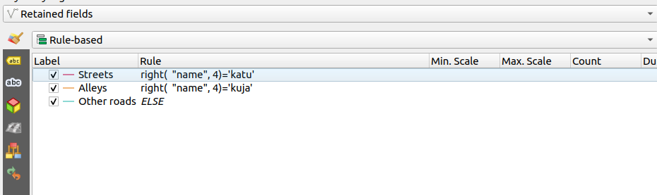
Let’s color the street network based on streetname endings: ‘katu’ = street, ‘kuja’ = alley, and a generic class for the rest. Since these are categories with no clear hierarchy, a quolitative color scheme fits our data the best.

Again, we’ll use expression, but this time rely on rule-based styling.

1. Select Rule-based as the styling type for the line layer.

2. Add two more line features. Copy the style of the first feature and paste it onto the other two (Copy symbol > Paste symbol).

3. Edit the first feature. Name it Streets. In filter, paste right("name", 4)='katu'. Use whatever color you wish: the example color is a bright red #d40a47.

   1. The filter matches the last four characters from the streetname column with katu (street). If there’s a match, the rule is applied.

   2. Paste the color hex code to: Color > Choose color… > HTML notation field.

4. Repeat for class #2.

   1. Name: Alleys

   2. Filter: right("name", 4)='kuja'

   3. Example color: #e78119

5. And the final class

   1. Name: Other roads

   2. No filter: Select Else: Catch-all for other features

   3. Example color: #30bab0

Now, your style panel should look something like the picture below

Layout

Next, it’s time to layout the map and export it. There are a thousand ways to create a good, eye-catching maps! Below is one attempt, but you are given free-hands to experiment.

If you need a refresher on QGIS’ Map composer, check out the official training manual.

The line layer in this example uses the style: QGIS-files/example_street_network_style.qml

This is far from a perfect map, but it has some basic cartographic elements and features that are good to keep in mind when making your map. However, it is highly encouraged to experiment with feature and background colors, map elements and their placement. As you create this map, be particularly mindful of:

• The use of colors: Are the different classes sensible for the phenomena that you’re representing? Is the contrast between the classes and the background enough to distinguish everything?

• Layout and composition: Are the different elements in balance? Does some section have an excess of empty space?

• Map elements: Do you have the elements needed for this map? Are you giving the reader enough information (about the setting, the map theme, the scale of the map etc.)?

Stretch goal

Want to create a more coherent street map? You can add building footprints from OSM by repeating the QuickOSM query from before but using building as the key. Different things to consider:

• The new layer will affect the readability of the map, make it more busy. Consider ways to de-emphasize the street network

• How could you highlight a particular building, say, the Kamppi shopping centre? Consider approaches like highlighting the target building with color or adding transparency to all other buildings.

Replicating the processing flow of this notebook

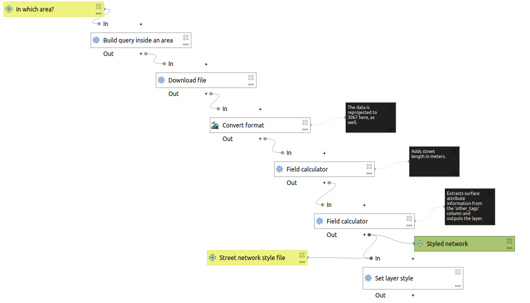
To get a street network file styled and ready for mapping, you may use this model file to replicate this process:

1. Download the style file and processing model in QGIS-files folder

2. In the top right corner of the Processing toolbox, select Open existing model and navigate to practical1_processing_steps.model3

3. Open the model and select example_street_network_style.qml as the Street network style file parameter. Run the model.

4. A new layer called Styled network has been added to the project.